Examples
This page shows example code snippets demonstrating how to use PulsarSA.
Configure workspace
The Workfolder for running the PulsarSA have the following structure to use the in-built methods:
work_folder/
├── payloads/ # folder for PulsarDT synthetic files
├── runtime/ # folder for PulsarDT simulation parameters log files
├── outputs/ # folder for generated results, outputs from the pipeline
├── models/ # folder for Pre-trained or trained model files
├── config_pipe.yml # Configuration file for pipeline setup
└── pipe_neural_network_models.py # neural network models definations
Details about the configuration file is provided below.
pipe_neural_network_models.py contains the neural network model definitions used in the pipeline. You can define your own models or use the pre-defined model UNet provided in PulsarSA.
Use the pipeline to detect pulsar signal from a single image
import numpy as np
from pulsarsa import PipelineImageToFilterToCCtoLabels
from pulsarsa.tools.example_neural_nets import ImageToMaskNetv3
#: Instantiate the pipeline
ppl2fensemble1 = PipelineImageToFilterToCCtoLabels(image_to_mask_network=ImageToMaskNetv3(),
trained_image_to_mask_network_path='./docs/example_dats/trained_cnn_eg_test_set_1_at_alpha.pt',
mask_filter_network=ImageToMaskNetv3(),
trained_mask_filter_network_path='./docs/example_dats/trained_cnnfilter_eg_test_set_1_at_alpha.pt',
snr_thresh=4,
box_func_window=5,
corr_thresh=2,
)
#: Load example data to test pulsar signal detection
example_fake_real_pulsar_data = np.load(file='./docs/example_dats/example_fake_real_pulsar_data.npy',mmap_mode='r')
image = example_fake_real_pulsar_data[9,:,:]
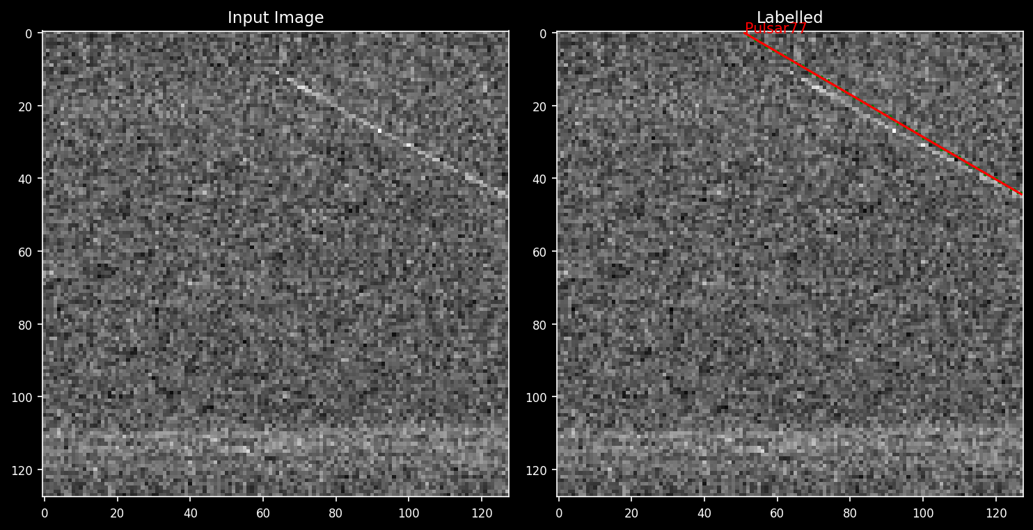
results = ppl2fensemble1(image=image)
ax = ppl2fensemble1.plot(image=image)
fig = ax[0].get_figure()
fig.savefig("./outputs/pipeline_output.png", dpi=150, bbox_inches="tight")
print(results)
output:
{'Pulsar': np.float64(77.0), 'Noise (NBRFI)': 0, 'Noise (BBRFI)': 0, 'Noise (None)': 0}
And the saved image output is:
Run pipeline PulsarSA
Synthetic Data Generation:
The PulsarDT simulation parameters are defined in the config_pipe.yml file. Below is the code snippets
from pulsarsa.tools.pipe_methods.data_gen_methods import generate_data_payloads_for_training,run_sample_plotter
generate_data_payloads_for_training(path_to_work_folder='./')
run_sample_plotter(path_to_work_folder='./')
or,
from pulsarsa.tools.pipe_methods import run_pipeline
run_pipeline(path_to_work_folder='./',
               need_data_gen=True,
               need_training=False,
               need_validation=False)
Training:
The PulsarSA training parameters are defined in the config_pipe.yml file. Below is the code snippets
from pulsarsa.tools.pipe_methods.training_methods import train_pipeline_neural_nets
train_pipeline_neural_nets(path_to_work_folder='./', skip_filter_training = False)
or,
from pulsarsa.tools.pipe_methods import run_pipeline
run_pipeline(path_to_work_folder='./',
               need_data_gen=False,
               need_training=True,
               need_validation=False)
Validation:
After training a pipeline instance can be loaded for pulse detection by the following script based on the congig_pipe.yml file:
from pulsarsa import PipelineImageToFilterToCCtoLabels
from pulsarsa.tools.pipe_methods.validation_methods import load_pipeline
pipeline_instance:PipelineImageToFilterToCCtoLabels = load_pipeline(path_to_work_folder='./') # Note for now only PipelineImageToFilterToCCtoLabels is supported
                                                                                              # for the following methods in this example
The PulsarSA validation parameters are defined in the config_pipe.yml file. Entries related to fil files are
validation:
   mlflow_folder: ./mlflows_validation/
   num_samples: 10
   path_to_metadata_file: ../data/metadata_file.csv
   path_to_real_filterbank_file: ../data/filterbank_file.fil
   random_seed:
   snr_band:
   - 10
   - 100
   resize_input: [128,128]
   time_window: 512
   position_column: position
   allow_randomness: 0
Entries related to npy files are:
validation:
   mlflow_folder: ./mlflows_validation/
   num_samples: 10
   path_to_metadata_npy_file:    ../docs/example_dats/example_fake_real_pulsar_data_label.npy
   path_to_real_npy_file: ../docs/example_dats/example_fake_real_pulsar_data.npy
   random_seed:
   resize_input: [128,128]
   allow_randomness: 0
Below is the code snippets
from pulsarsa.tools.pipe_methods.validation_methods import validate_pipeline
validate_pipeline(path_to_work_folder='./',file_type='npy') # In future versions fil mode will be preffered
or,
from pulsarsa.tools.pipe_methods import run_pipeline
run_pipeline(path_to_work_folder='./',
               need_data_gen=False,
               need_training=False,
               need_validation=True
               val_file_type='npy')
Running the above code prints the performance metrics in terminal as shown below:
F1 Score: 1.0, Accuracy: 1.0, Precision: 1.0, Recall: 1.0
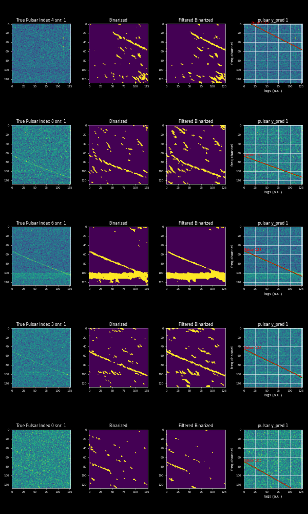
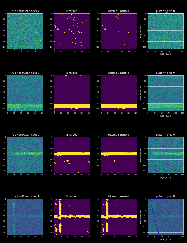
Running the above script also saves 5 plots of pulse detections and non-pulse detections as shown below.
Running the above script also saves 5 plots of pulse and non-pulse detections shown below.
Pulse Detections
Non-Pulse Detections
Also it activates the mlflow logging in a folder defined in config_pipe.yml for validation. Therefore multiple runs can be visualized using mlflow for detailed information.
For running the pipeline as a whole all keys related to each subprocess of the pipeline can be set to True like below
from pulsarsa.tools.pipe_methods import run_pipeline
run_pipeline(path_to_work_folder='./',
               need_data_gen=True,
               need_training=True,
               need_validation=True)
Fine Tuning:
Fine tuning of pipeline parameters like ‘min_axis_ratio’, ‘min_cc_size_threshold’, ‘box_func_window’ etc can be tuned for the best performance scores. This can be acheived by defining a dict called param_grid where possible values of such parameters can be defined and the function run_pipeline_estimator_on_paramgrid will return the parameter mix for the best performance scores.
Below is the code snippet:
from pulsarsa.tools.pipe_methods.parameter_tuning import run_pipeline_estimator_on_paramgrid
param_grid = {'min_axis_ratio':[4,5],
     'min_cc_size_threshold':[10,11,12],
     'box_func_window':[3,4,5]}
best_params = run_pipeline_estimator_on_paramgrid(path_to_work_folder='./',param_grid=param_grid,file_type='npy')
print(best_params)
this will return:
{'best_F_score_param': {'min_axis_ratio': 4, 'min_cc_size_threshold': 10, 'box_func_window': 3, 'score': 1.0},
 'best_accuracy_param': {'min_axis_ratio': 4, 'min_cc_size_threshold': 10, 'box_func_window': 3, 'score': 1.0},
  'best_precision_param': {'min_axis_ratio': 4, 'min_cc_size_threshold': 10, 'box_func_window': 3, 'score': 1.0},
   'best_recall_param': {'min_axis_ratio': 4, 'min_cc_size_threshold': 10, 'box_func_window': 3, 'score': 1.0}}
Fine tuning is also possible, incase we have pipelines trained on different types of simulation datasets. The idea is use the Principal component analysis (PCA) to find the principal components (PCs) to later mix the pipelines (basically the NN models used in the pipelines) to come up with the best of all pipelines. This can be acheived with the following code below
Below is the code snippet:
from pulsarsa.tools.pipe_methods.validation_methods import load_pipeline
from pulsarsa.tools.pipe_methods.parameter_tuning import run_pipeline_estimator_on_pca_componentgrid

pipeline0 = load_pipeline('./ensemble0/')
pipeline1 = load_pipeline('./ensemble1/')

best_params = run_pipeline_estimator_on_pca_componentgrid(pipelines=[pipeline0,pipeline1],
                                                          PCA_grid_resolution=0.1,
                                                          variance_to_capture=1,
                                                          path_to_work_folder='./',
                                                          file_type='npy')

print(best_params)
this will return:
{'best_F_score_param': {'PC0': np.float64(-0.9), 'score': 1.0},
'best_accuracy_param': {'PC0': np.float64(-0.9), 'score': 1.0},
'best_precision_param': {'PC0': np.float64(-1.0), 'score': 1.0},
'best_recall_param': {'PC0': np.float64(-0.9), 'score': 1.0}}
Subsequent examples are focused more on the applications of the core PulsarSA and PulsarDT function and methods.
Generate data for training
from pulsardt import generate_example_payloads_for_training
generate_example_payloads_for_training(tag='train_set_1_',
                                     num_payloads=1000,
                                     freq_channels = np.arange(0.42, .85, 0.0025),
                                     rot_phases= (0, 360*1, 1),
                                     antenna_sensitivity=0.5,
                                     plot_a_example=False,
                                     param_folder='./syn_data/runtime/',
                                     payload_folder='./syn_data/payloads/',
                                     num_cpus=10, #: choose based on the number of nodes/cores in your system,
                                     prob_bbrfi=0.2,
                                     prob_nbrfi=0.2,
                                     )
Train a neural network
import numpy as np
from pulsarsa import PrepareFreqTimeImage, ImageToMaskDataset, TrainImageToMaskNetworkModel
from pulsarsa.tools.example_neural_nets import ImageToMaskNetv3
from pulsarsa.neural_network_models import WeightedBCELoss
#: Instantiate the trainer
image2mask_network_trainer = TrainImageToMaskNetworkModel(
model=ImageToMaskNetv3(),
num_epochs=20,
store_trained_model_at="./syn_data/model/trained_net_test.pt",
loss_criterion = WeightedBCELoss(pos_weight=3,neg_weight=1)
)
#: Define datasets and dataloaders
image_loader = PrepareFreqTimeImage(
do_rot_phase_avg=True,
do_binarize=False,
do_resize=True,
resize_size=(128,128),
)
mask_loader = PrepareFreqTimeImage(
do_rot_phase_avg=True,
do_binarize=True,
do_resize=True,
resize_size=(128,128),
)
image_tag='train_set_1_*_payload_detected.json'
image_directory='./syn_data/payloads/'
mask_tag = 'train_set_1_*_payload_flux.json'
mask_directory='./syn_data/payloads/'
image_mask_dataset = ImageToMaskDataset(
image_tag = image_tag,
mask_tag= mask_tag,
image_directory = image_directory,
mask_directory = mask_directory,
image_engine=image_loader,
mask_engine=mask_loader
)
#: Start training
image2mask_network_trainer(image_mask_pairset=image_mask_dataset)
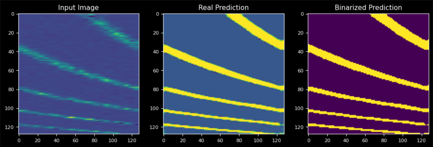
#: Plot prediction
idx = int(np.random.rand()*1000)
image = image_mask_dataset[idx][0]
image2mask_network_trainer.test_model(image=image,plot_pred=True)
Use Tuner to manually tune mixed pipelines (Note: This part needs to be run in notebook)
Node 1 of the notebook should contain the following code to instantiate the tuner:
from pulsarsa import PipelineImageToFilterToCCtoLabels
from pulsarsa.tools.example_neural_nets import ImageToMaskNetv3

#: Instantiate 4 pipelines trained on different dataset ensembles
ppl2fensemble0 = PipelineImageToFilterToCCtoLabels(image_to_mask_network=ImageToMaskNetv3(),
                             trained_image_to_mask_network_path='./docs/example_dats/trained_cnn_eg_test_set_0_at_alpha.pt',
                             mask_filter_network=ImageToMaskNetv3(),
                             trained_mask_filter_network_path='./docs/example_dats/trained_cnnfilter_eg_test_set_0_at_alpha.pt',
                             )

ppl2fensemble1 = PipelineImageToFilterToCCtoLabels(image_to_mask_network=ImageToMaskNetv3(),
                             trained_image_to_mask_network_path='./docs/example_dats/trained_cnn_eg_test_set_1_at_alpha.pt',
                             mask_filter_network=ImageToMaskNetv3(),
                             trained_mask_filter_network_path='./docs/example_dats/trained_cnnfilter_eg_test_set_1_at_alpha.pt',
                             )

#: Instantiate the tuner
tn = Tuner(sample_of_objects=[ppl2fensemble0,ppl2fensemble1],reset_components=False,variance_to_capture=2,all_sliders=True)

To get the slider functionality run it in a jupyter notebook with all_sliders=True

The mixed neural nets can be saved in the folder as shown below in the next node block:
ppl2fmixed = tn(folder_to_save='./syn_data/model/')
in script mixed pipeline can be created by passing the normalized PCA factors (having range (-1.0 to 1.0)) as:
ppl2fmixed = tuner.generate_mixed_model_from_input_pca_factors([-0.9,0])